Modelling with functions and equations
In this module we consider modelling simple relations using
variables, functions and equations. These are the most fundamental
mathematical tools.
Before the problems begin:
- Read all general
instructions carefully.
- Look at the Mathematica
hints.
- For the quality of your presentation, see the writing
hints for some help and suggestions.
- General hint: The first part of problem solving is to understand the problem. It is always good to spend time to really understand the problem, before trying to solve it!
Remember
- This is not a distance learning course! The problems are deliberately phrased so that it is not obvious
what the "correct" approach is. Asking questions and discussing your ideas in supervision is an important part of this course.
- Be sure to apply the self check before you submit.
- Follow the submission instructions carefully.
- Do not search for solutions, it is not the
correct answer that is most important, and you do not need it to pass. Do not spread your solutions or other insights to
other groups! Indicate any external source.
- It is up to you
to plan how much work you want to spend on each problem, as well as to
consider when
you have arrived at a reasonable answer.
In your
solutions:
- Make reasonable assumptions to make the question as precise as
you need.
- Even if you do not fully solve the problem, report what you have
done in a clear and logically consistent way, including observations,
hypotheses, failed attempts etc. Show that you really tried.
- Make sure you that you answer the right question! A clear and
precise answer is always best if possible, otherwise consider a partial
answer or a discussion. Take care to perform all tasks and answer every question
written in a particular problem.
- (FORMULAS PROBLEM) A number of mathematical equations are listed below.
A common thing to look at when you see an expression is its
mathematical form, e.g. continuous/discrete, linear/nonlinear etc. This
is extensively discussed in mathematics courses. However, such
observations have to do only with the properties of the expression
itself, and is like studying the grammar of a sentence rather than its
meaning. In contrast, mathematical modelling is about how to say
something about reality by using mathematical expressions, and this is
what I want you to think about in this problem.
For each equation discuss what the justification of the equation is
(how do we know it is true or at least reasonable), and how well it can
be
expected to fit with reality (i.e. is it exact or is it some kind of
approximation). If you can, try to categorize the
expressions in different groups. Since this is the first problem in
the course, a hint is not to spend all your time here since you have
more problems in this set. A short comment on each equation and maybe
a few general observations is sufficient.
- a^2+b^2=c^2 (Pythagoras theorem)
- stock index= 2045+0.0034 t (trend analysis)
- population= C * a^t (C and a are constants, t is the time
in
years)
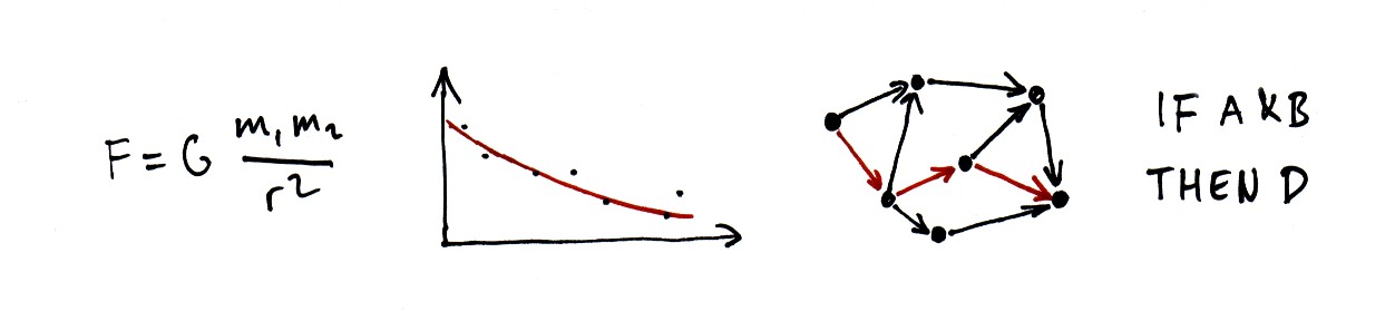
- F= G m1 m2 / r^2 (gravity between two bodies)
- F=ma (Newtons force equation)
- 100*weight+length < 320 (max allowed parcel size for a
postal service)
- #presentStudents + #absentStudents = #allStudents (for a
class)
- I1+I2+I3=0 (total electric current into a circuit knot)
- insurance rebate in % = #insurances *2 + 0.2* min(7, #years as
customer) (lower rates for good customers)
- (a+b)^2 = a^2 + 2ab + b^2
- A >= 0.08 * L * I (dimensioning requirement for
12V cables if you have a current I [A], cable length L[m] and cable
area A[mm^2])
- air drag force = C* v^2 * A (air drag for a moving object,
C is a constant depending on the shape but not the size, v velocity, A
cross section
area)
- weight = C* length^3 (the constant C should be chosen
depending on type of object e.g. persons, dogs, cars)
- p(getting heads when tossing a coin) = 1/2
- (INTUITIVE CURVE FITTING PROBLEM) For two related physical variables the following relationship has been measured:
T (time)
|
D (distance)
|
88.0
|
57.9
|
224.7
|
108.2
|
365.3
|
149.6
|
687.0
|
228.07
|
4332
|
778.434
|
10760
|
1428.74
|
30684
|
2839.08
|
60188
|
4490.8
|
90467
|
5879.13
|
{{88.0, 57.9},{224.7,108.2},{365.3,149.6},{687.0,228.07},{4332,
778.434},{10760,
1428.74},{30684,2839.08},{60188,4490.8},{90467,5879.13}}
Suggest a mathematical equation describing the relation between these
two quantities. Feel free to use your creativity, any method to get to
a good result is fine. Explain how you did to find the model, and
motivate your choice. Is the fit of your equation good? How can
deviations from the known table entries be justified? How could the
model you found be used for points not in the table, e.g. for other
values of T? Hint: Make sure you get started by doing something.
Plot the points, plot some functions and explore all possibilities you
can think of. What you definitely shouldn't do is to try to look
up an answer, or use some software that searches automatically - it is
your own exploration that is important.
You don't have to use Mathematica for this problem but if you want to
plot the data points in Mathematica you can use ListPlot. If you want
to superimpose a function and the points in the same diagram you can
use Show with Plot[your function] and ListPlot[the data] as arguments.
Look in the Mathematica help system for extensive documentation and
examples.
- (PENDULUM PROBLEM) Use dimensional analysis to find a mathematical expression for the
period of a pendulum. Begin by setting up variables that could be
expected to affect the period, and determine their dimension. Explain
the solution process
and how you arrive to the conclusion. Make a little experiment to verify your
result, and estimate any unknown proportionality constant (don't forget this
last step to make the
task complete!).
NOTE: Avoid getting involved in complicated physics here. This is
not the task. The task is simply to guess a formula based on dimensional
correctness only! If you don't understand what this is, stop and ask. If you already know the answer, part of the purpose of
the problem is lost, then ask us and we will find an alternative for you. Please
do the same also for other problems in the course if you realize that
you already know the answer.
- (BICYCLE BRAKING PROBLEM) According to an experiment with a bicycle the following stopping
distances were measured:
speed [km/h]
|
stopping distance [m]
|
5
|
0.65
|
10
|
1.3
|
15
|
2.7
|
20
|
5.1
|
22
|
5.6
|
25
|
7.4
|
30
|
10.4
|
{{5, 0.65}, {10, 1.3}, {15, 2.7}, {20, 5.1}, {22, 5.6}, {25, 7.4}, {30,
10.4}}
a) This problem is about how to best fit a curve to given data. To get the basic idea of something and improve understanding, it is often good to start with a very simple example. So first try to manually fit a quadratic function to the points (1,3), (2,2), (3,4). Start by writing the equations that you know should hold, and then solve for the unknown parameters. When you see how this is done, add one more point (4,5). What happens?
Now consider the least squares method. Describe the idea of linear least squares as well as you can (see the paper available as additional course material, note that "linear least squares" is a special case of the least squares
method). Why is the least squares method meaningful only in the case
when you have more data points than parameters? What happens otherwise?
What does the Mathematica function Fit do?
b) Fit a straight line to the data using the least squares criterion
(this is yet another special case called linear regression and is very
common). Discuss the quality of the model.
c) Propose and motivate a better model for the distance as a function
of the speed, and fit it to the table entries. If you can, motivate
your model theoretically, and not only empirically. How would you judge
the quality of the fit? How can deviations from the known table entries
be justified? Could this model be reliably used for new points
not in the table? Try to draw as many conclusions of the data and your
model as you can.
- (SPLINES PROBLEM) Now we will consider curve fitting that passes exactly through the
data points. We will use the same stopping distance data as in the
previous problem.
a) Polynomial series can be used to approximate any function with
arbitrary precision. Use a polynomial of sufficiently high degree to
fit the
given
points in problem 4 exactly. What degree should that polynomial have
and why?
What does the result look like?
b) A common technique for curve fitting that passes exactly through
given data points is linear and cubic spline interpolation. Make sure
you first understand the essential points, without getting lost
in unnecessary details (see the lecture slide). If you feel
you need to learn more about this look in a book or see for example
- Brief mathematical descriptions: link1,
link2,
link3,
link4 (look for others if you like!)
- An app
where you can construct cubic splines through a given set of points. Cubic splines are called "natural" splines in this app.
Briefly explain the mathematical idea of spline interpolation (you are
not required to actually compute a spline for the example). Why is
spline interpolation often better than high degree polynomials for
exact curve fitting?
c) Compare
exact curve fitting (splines) with approximate model
fitting using the least squares
method (as in problem 4). Try to indicate advantages and
disadvantages with the respective methods. Consider both
the situation when you have many
accurate data points and when you have few data points and/or data of
very
low quality.
d) All smooth computer graphics is based on splines. The letters you
see on the screen, the curves in a graphics program. If we want to
describe an arbitrary 2-D curve, could we
use the cubic spline approach as in b) directly? Think for example of
drawing an 8. (If you don't
get it you may skip this question)
- (SURPRISE PROBLEM) Say that we would like to put a number on how surprised we get when
we see something happen. For example, when the sun goes up in the
morning we are not surprised at all, and if it didn't we would be very
surprised. If you think about it you will surely come to the conclusion
that there are many factors in your understanding of the world that
influences your degree of surprise. However, an interesting idea is
that all these factors can be summarized in a single number, namely
your estimate of the probability that a particular event will happen,
p(event).
We will not consider how to estimate this number. However, if this can
be done, we can ask ourselves which function surprise(p) we should then
use to calculate our level of surprise?
a) As a first step, use your intuition to suggest the extreme points
of this function.
b) Now consider the following intuitive argument. If we see two
unrelated events A and B happen, it seems reasonable that the sum of
the surprises of these two events independently should be equal to the
surprise of the
single combined event A AND B. If you also take this into account,
what function do you propose?
SELF-CHECK
- Have you answered all questions to the best of your ability?
- Is all the required information on the front page, is the file name correct etc.? (See here)
- Anything else you can easily check? (details, terminology, arguments, clearly stated answers etc.?)
Do not submit an incomplete module! We are available to help you, and you can receive a short extension if you contact us.